Gradient Descent for Logistic Regression in Python

Gradient descent (GD) is by far the most popular optimization strategy used in machine learning and deep learning at the moment. It is used when training data models, can be combined with every algorithm and is easy to understand and implement. Everyone working with machine learning should understand its concept. We’ll walk through how to implement the gradient descent algorithm in an artificial neuron pf our own.

Notes

1. Import libraries

• numpy for mathematical operations
• matplotlib for data visualization
• sklearn.datasets for work on it
• accuracy_score for evaluation

import numpy as np
import matplotlib.pyplot as plt
from sklearn.datasets import make_blobs

from sklearn.metrics import accuracy_score

Personalize graph

plt.style.use('dark_background')
plt.rcParams.update({
    "figure.facecolor":  (0.12 , 0.12, 0.12, 1),
    "axes.facecolor": (0.12 , 0.12, 0.12, 1),
})

Let’s generate some data to practice with the make_blobs function from sklearn.dataset by specifying the number of inputs, the number of features, the centers and the random state

# Generate data to practice
X, y = make_blobs(n_samples=100, n_features=2, centers=2, random_state=0)

# reshaping for a better adaptation to the calculation
y = y.reshape((y.shape[0], 1))

print('Dimension of X:', X.shape)
print('Dimension of y:', y.shape)

plt.scatter(X[:,0], X[:, 1], c=y, cmap='prism')
plt.show()

Dimension of X: (100, 2)
Dimension of y: (100, 1)

2.Define Functions

Initialization

In order to create the initialization parameters of our separation line, i.e. different weights of the synaptic connections as well as the bias, the whole from the generated sample data

def initialization(X):
    W = np.random.randn(X.shape[1], 1)
    b = np.random.randn(1)
    return (W, b)

Model creation

To create the equations of the separation line and the activation function that will allow us to make better predictions. This function returns the active input

def model(X, W, b):
    Z = X.dot(W) + b
    A = 1 / (1 + np.exp(-Z))
    return A

Logarithmic Loss

In order to determine how close or far we are from the exact value after our prediction

def log_loss(A, y):
    return 1 / len(y) * np.sum(-y * np.log(A) - (1 - y) * np.log(1 - A))

Gradient

To apply more efficiently the equations related to gradient descent

def gradients(A, X, y):
    dW = 1 / len(y) * np.dot(X.T, A - y)
    db = 1 / len(y) * np.sum(A - y)
    return (dW, db)

Update Function

To apply the gradient descent

def update(dW, db, W, b, learning_rate):
    W = W - learning_rate * dW
    b = b - learning_rate * db
    return (W, b)

Predict Function

To predict the class of an input

def predict(X, W, b):
    A = model(X, W, b)
    print(A)
    return A >= 0.5

3. Create a Neuron

def artificial_neuron(X, y, learning_rate = 0.1, n_iter = 150):

    # Initialization W, b
    W, b = initialization(X)

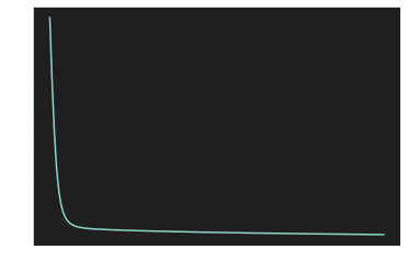
    Loss = []

    # Iteration loop
    for i in range(n_iter):
        A = model(X, W, b)
        Loss.append(log_loss(A, y))
        dW, db = gradients(A, X, y)
        W, b = update(dW, db, W, b, learning_rate)

    y_pred = predict(X, W, b)
    print(accuracy_score(y, y_pred))
    
    plt.plot(Loss)
    plt.show()

    return (W, b)

4.Visualization of the learning curve

W, b = artificial_neuron(X, y)

[[9.80406021e-01]
 [7.67042239e-01]
 [3.40212232e-03]
 [1.12525858e-01]
 [9.75128801e-01]
 [3.45771392e-01]
 [6.01324891e-02]
 [9.67989464e-01]
 [3.78178879e-02]
 [8.76950867e-01]
 [2.42449942e-02]
 [8.88622356e-01]
 [2.13762006e-02]
 [1.24436424e-02]
 [7.41091849e-01]
 [9.90674953e-01]
 [9.94228232e-01]
 [2.71722474e-02]
 [7.26832689e-01]
 [6.53086468e-01]
 [3.81186926e-02]
 [2.84476759e-02]
 [3.89230890e-01]
 [3.35613428e-03]
 [9.63415884e-01]
 [2.57800801e-02]
 [9.00335852e-01]
 [6.60403491e-03]
 [5.91310866e-02]
 [7.80684024e-01]
 [9.83746413e-01]
 [3.66461272e-02]
 [6.68889861e-01]
 [9.84074985e-01]
 [4.10732753e-01]
 [2.41459372e-01]
 [7.92174340e-01]
 [5.77816615e-01]
 [4.95755288e-01]
 [4.29962960e-01]
 [5.10137463e-02]
 [7.64492353e-02]
 [4.79641209e-04]
 [1.56666125e-01]
 [1.79877131e-01]
 [8.65087917e-01]
 [9.73102525e-01]
 [9.66838846e-01]
 [2.83194027e-03]
 [6.89536120e-03]
 [9.49692444e-01]
 [5.48293144e-01]
 [4.59304399e-02]
 [3.52285969e-02]
 [8.62738290e-01]
 [3.57490916e-02]
 [7.62844063e-01]
 [8.40989205e-01]
 [9.63965862e-01]
 [9.93446898e-01]
 [6.61394544e-01]
 [1.82090079e-01]
 [3.23128502e-03]
 [9.44445420e-01]
 [1.15292589e-02]
 [3.68069696e-01]
 [2.62313035e-02]
 [6.74894046e-01]
 [9.59434717e-01]
 [2.76641732e-01]
 [1.65157243e-01]
 [9.29801123e-01]
 [9.81566397e-01]
 [1.06083626e-01]
 [9.58192444e-02]
 [2.87442858e-02]
 [5.24151565e-01]
 [8.97775539e-01]
 [3.70343678e-02]
 [2.80549476e-02]
 [2.62000271e-01]
 [8.94007894e-02]
 [2.67674156e-03]
 [1.11281924e-01]
 [8.11706942e-02]
 [8.72276677e-03]
 [9.79280903e-01]
 [6.77017113e-02]
 [8.19492552e-01]
 [9.67327252e-01]
 [9.24699396e-01]
 [9.86395708e-01]
 [4.45440388e-01]
 [9.33605778e-01]
 [3.39032074e-01]
 [6.16076544e-04]
 [9.80401775e-01]
 [9.73055392e-01]
 [6.16480769e-03]
 [4.11420426e-01]]
0.89

print(W, b)

[[ 1.42330917]
 [-1.1221567 ]] [0.41562285]

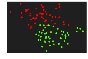
Let’s visualize and predict the class of a new element

element = np.array([2,1])

plt.scatter(X[:,0], X[:, 1], c=y, cmap='prism')
plt.scatter(element[0], element[1], c='blue')

plt.show()
print(predict(element, W, b))

[0.89473857]
[ True]

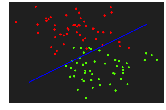
5. Descision border

Render the descision frontier

fig, ax = plt.subplots(figsize=(9, 6))
ax.scatter(X[:,0], X[:, 1], c=y, cmap='prism')

x1 = np.linspace(-1, 4, 100)
x2 = ( - W[0] * x1 - b) / W[1]

ax.plot(x1, x2, c='blue', lw=3)

[<matplotlib.lines.Line2D at 0x7f2c76337e80>]

6. 3D Visualization

import plotly.graph_objects as go

fig = go.Figure(data=[go.Scatter3d( 
    x=X[:, 0].flatten(),
    y=X[:, 1].flatten(),
    z=y.flatten(),
    mode='markers',
    marker=dict(
        size=5,
        color=y.flatten(),                
        colorscale='YlGn',  
        opacity=0.8,
        reversescale=True
    )
)])

fig.update_layout(template= "plotly_dark", margin=dict(l=0, r=0, b=0, t=0))
fig.layout.scene.camera.projection.type = "orthographic"
fig.show()

X0 = np.linspace(X[:, 0].min(), X[:, 0].max(), 100)
X1 = np.linspace(X[:, 1].min(), X[:, 1].max(), 100)
xx0, xx1 = np.meshgrid(X0, X1)
Z = W[0] * xx0 + W[1] * xx1 + b
A = 1 / (1 + np.exp(-Z))

fig = (go.Figure(data=[go.Surface(z=A, x=xx0, y=xx1, colorscale='YlGn', opacity = 0.7, reversescale=True)]))

fig.add_scatter3d(x=X[:, 0].flatten(), y=X[:, 1].flatten(), z=y.flatten(), mode='markers', marker=dict(size=5, color=y.flatten(), colorscale='YlGn', opacity = 0.9, reversescale=True))


fig.update_layout(template= "plotly_dark", margin=dict(l=0, r=0, b=0, t=0))
fig.layout.scene.camera.projection.type = "orthographic"
fig.show()

Links

Getting The Code On Google Colab

The entire code containing all the code mentioned in this post can be found here.

Getting The Code On Github

The entire folder containing all the code mentioned in this post can be found via this link.

Just bear in mind that you will need to install all the dependencies. If you find any issues with the code, feel free to either comment down below or raise an issue on Github.

Add me on LinkedIn

Don’t hesitate to follow me on linkedIn or o other social network to encourage me to do more posts on IT.