Cats vs Dog with Logistic Regression using Gradient Descent in Python

In this article, we’ll be going to make our first project of prediction of cats or dogs from their respective images using Logistic Regression. We are going to use scikit-learn library for this project to create a sample dataset with make_blobs.

The main focus of this sample project is towards data collection, data preprocessing and mathematics knowledges application rather than training a Logistic Regression model. The reason is that I showed how to set different hyperparameters in order to achieve satisfying results and often times whenever working on a project 80% of the time one gonna spent is on data preprocessing.

The project is going to be a Jupyter Notebook. Everything you need from code to explanation is already provided in this notebook. This article will tell you few points about the dataset and some techniques we are going to use.

Notes

1. Import libraries

• numpy for mathematical operations
• matplotlib for data visualization
• sklearn.datasets for work on it
• accuracy_score for evaluation
• tqdm for the progression bar

import numpy as np
import matplotlib.pyplot as plt

from sklearn.datasets import make_blobs
from sklearn.metrics import accuracy_score

from tqdm import tqdm

Personalize pyplot graph by setting a background color and a facecolors.

plt.style.use('dark_background')
plt.rcParams.update({
    "figure.facecolor":  (0.12 , 0.12, 0.12, 1),
    "axes.facecolor": (0.12 , 0.12, 0.12, 1),
})

2. Define functions

Initialization

In order to create the initialization parameters of our separation line, i.e. different weights of the synaptic connections as well as the bias, the whole from the generated sample data.

def initialisation(X):
    W = np.random.randn(X.shape[1], 1)
    b = np.random.randn(1)
    return (W, b)

Model Creation

To create the equations of the separation line and the activation function that will allow us to make better predictions. This function returns the active input.

def model(X, W, b):
    Z = X.dot(W) + b
    # print(Z.min())
    A = 1 / (1 + np.exp(-Z))
    return A

Logarithmic Loss

In order to determine how close or far we are from the exact value after our prediction to which we have added an epsilon parameter so that this logarithmic function can be computed and approximated even when our input values tend to 0 because the latter is not defined there.

def log_loss(A, y):
    epsilon = 1e-15
    return 1 / len(y) * np.sum(-y * np.log(A + epsilon) - (1 - y) * np.log(1 - A + epsilon))

Gradient

To apply more efficiently the equations related to gradient descent.

def gradients(A, X, y):
    dW = 1 / len(y) * np.dot(X.T, A - y)
    db = 1 / len(y) * np.sum(A - y)
    return (dW, db)

Update function

To apply the gradient descent to improve the efficience of the model.

def update(dW, db, W, b, learning_rate):
    W = W - learning_rate * dW
    b = b - learning_rate * db
    return (W, b)

Predict function

To predict the class of an input.

def predict(X, W, b):
    A = model(X, W, b)
    # print(A)
    return A >= 0.5

3. Create an Artificial Neuron

It is mainly the function used for our previous logistic regression model that we have improved for a better training of artificial neuron models in order to produce more detailed graphs in relation with its learning curve.

def custom_artificial_neuron(X_train, y_train, X_test, y_test, learning_rate = 0.1, n_iter = 100):

    # initialization W, b
    W, b = initialization(X_train)

    train_loss = []
    train_acc = []
    test_loss = []
    test_acc = []

    for i in tqdm(range(n_iter)): # Progession bar
        A = model(X_train, W, b)

        if i %10 == 0: # condition to reduce the computation and the speed of the algorithm
            # Train
            train_loss.append(log_loss(A, y_train))
            y_pred = predict(X_train, W, b)
            train_acc.append(accuracy_score(y_train, y_pred))

            # Test
            A_test = model(X_test, W, b)
            test_loss.append(log_loss(A_test, y_test))
            y_pred = predict(X_test, W, b)
            test_acc.append(accuracy_score(y_test, y_pred))

        # update
        dW, db = gradients(A, X_train, y_train)
        W, b = update(dW, db, W, b, learning_rate)


    plt.figure(figsize=(12, 4))
    plt.subplot(1, 2, 1) # Train graph
    plt.plot(train_loss, label='train loss')
    plt.plot(test_loss, label='test loss')
    plt.legend()
    plt.subplot(1, 2, 2)  # Accuracy graph
    plt.plot(train_acc, label='train acc')
    plt.plot(test_acc, label='test acc')
    plt.legend()
    plt.show()

    return (W, b)

4. Application: Cat vs Dog classification

Import dependencies

!pip install h5py #This line is required if you are using a jupyter notebook or other software on your computer
from utilities import * # To load  data in a jupyter notebook or other software 

Defaulting to user installation because normal site-packages is not writeable
Collecting h5py
  Downloading h5py-3.7.0-cp39-cp39-manylinux_2_12_x86_64.manylinux2010_x86_64.whl (4.5 MB)
     ━━━━━━━━━━━━━━━━━━━━━━━━━━━━━━━━━━━━━━━━ 4.5/4.5 MB 907.6 kB/s eta 0:00:00m eta 0:00:01[36m0:00:01
[?25hRequirement already satisfied: numpy>=1.14.5 in /usr/lib/python3/dist-packages (from h5py) (1.19.5)
Installing collected packages: h5py
Successfully installed h5py-3.7.0

Load data

X_train, y_train, X_test, y_test = load_data()

print(X_train.shape)
print(y_train.shape)
print(np.unique(y_train, return_counts=True))

(1000, 64, 64)
(1000, 1)
(array([0., 1.]), array([500, 500]))

print(X_test.shape)
print(y_test.shape)
print(np.unique(y_test, return_counts=True))

(200, 64, 64)
(200, 1)
(array([0., 1.]), array([100, 100]))

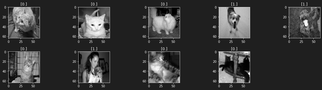
Visualize labeled data form the dataset

plt.figure(figsize=(16, 8))
for i in range(1, 10):
    plt.subplot(4, 5, i)
    plt.imshow(X_train[i], cmap='gray')
    plt.title(y_train[i])
    plt.tight_layout()
plt.show()

/usr/local/lib/python3.7/dist-packages/matplotlib/text.py:1165: FutureWarning: elementwise comparison failed; returning scalar instead, but in the future will perform elementwise comparison
  if s != self._text:

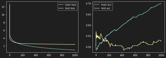
5. Training the model

Flatten and normalize data

We flatten our data because our model is designed to work on inputs with 2 features or 2 dimensions while the shape of (1000, 64, 64) is 3 dimensions.

So to be usable in our model, we have to reshape and normalize them to avoid that our gradient descent algorithm makes too big jumps depending on one of its input features, preventing it from reaching the global minimum of our log_loss function

Train set reshape

X_train_reshape = X_train.reshape(X_train.shape[0], -1) / X_train.max()
X_train_reshape.shape

(1000, 4096)

X_test_reshape = X_test.reshape(X_test.shape[0], -1) / X_train.max()
X_test_reshape.shape

(200, 4096)

W, b = artificial_neuron(X_train_reshape, y_train, X_test_reshape, y_test, learning_rate = 0.01, n_iter=10000)

100%|████████████████████████████████████| 10000/10000 [01:35<00:00, 104.48it/s]

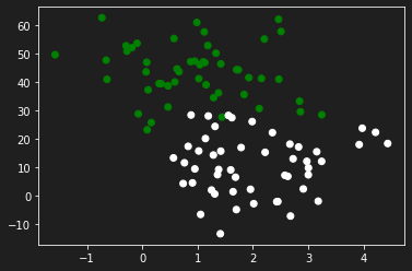
6. Normalization: Why is it so important ?

In machine learning as well as in deep learning, data normalization is very important. Indeed, it intervenes in order to avoid that the input parameters of the model having a predominant impact on the output(s), do not come to crush the most minor ones, thus compressing our cost function and consequently preventing a good convergence of our gradient descent algorithm. Let’s observe this with a little numerical experiment and descriptive diagrams.

i. Case of unstandardized data

Create a dataset

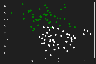
Let’s generate some data to practice with the make_blobs function from sklearn.dataset by specifying the number of inputs, the number of features, the centers and the random state.

In this particular case we will propose a configuration of features in which a specific parameter has an influence influence on the output than the other.

from sklearn.datasets import make_blobs

X, y = make_blobs(n_samples=100, n_features=2, centers=2, random_state=0)
X[:, 1] = X[:, 1] * 10

y = y.reshape(y.shape[0], 1)

plt.scatter(X[:,0], X[:, 1], c=y, cmap='ocean')
plt.show()

Create an experimental neuron

This artificial neuron will be used mainly to evaluate and visualize the evolution of the learning curve of our model according to the input data.

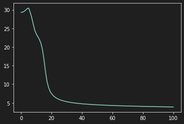
def experimental_neuron(X, y, learning_rate=0.1, n_iter=1000):

  W, b = initialization(X)
  W[0], W[1] = -7.5, 7.5

  nb = 1
  j=0
  history = np.zeros((n_iter // nb, 5))

  A = model(X, W, b)
  Loss = []
  

  Params1 = [W[0]]
  Params2 = [W[1]]
  Loss.append(log_loss(y, A))
  
  # Training
  for i in range(n_iter):
    A = model(X, W, b)
    Loss.append(log_loss(y, A))
    Params1.append(W[0])
    Params2.append(W[1])
    dW, db = gradients(A, X, y)
    W, b = update(dW, db, W, b, learning_rate = learning_rate)

    if (i % nb == 0):  
      history[j, 0] = W[0]
      history[j, 1] = W[1]
      history[j, 2] = b
      history[j, 3] = i
      history[j, 4] = log_loss(y, A)
      j +=1

  plt.plot(Loss)
  plt.show()

  return history, b, Loss, Params1, Params2

Visualization of the learning curve

history, b, Loss, Params1, Params2 = experimental_neuron(X, y, learning_rate=0.6, n_iter=100)

/usr/local/lib/python3.7/dist-packages/ipykernel_launcher.py:4: RuntimeWarning:

overflow encountered in exp

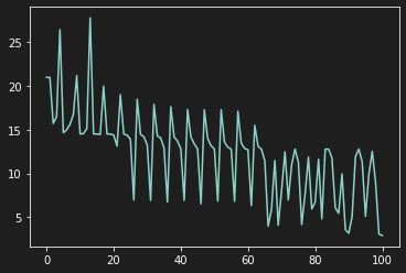
As we can see on the previous graph, our model learns in a very tumultuous way because the features do not have the same scale.

Visualize Gradient Descent Implementation

Import dependencie

from matplotlib.animation import FuncAnimation

Define a range of parameters

lim = 15
h = 100
W1 = np.linspace(-lim, lim, h)
W2 = np.linspace(-lim, lim, h)

W11, W22 = np.meshgrid(W1, W2)

W_final = np.c_[W11.ravel(), W22.ravel()].T
W_final.shape

(2, 10000)

Let’s take the equations of our neural network

Z = X.dot(W_final) + b
A = 1 / (1 + np.exp(-Z))

epsilon = 1e-15
L = 1 / len(y) * np.sum(-y * np.log(A + epsilon) - (1 - y) * np.log(1 - A + epsilon), axis=0).reshape(W11.shape)
L.shape

/usr/local/lib/python3.7/dist-packages/ipykernel_launcher.py:2: RuntimeWarning:

overflow encountered in exp

(100, 100)

Render Gradient Descent

Let’s define a function to graphically render the gradient descent

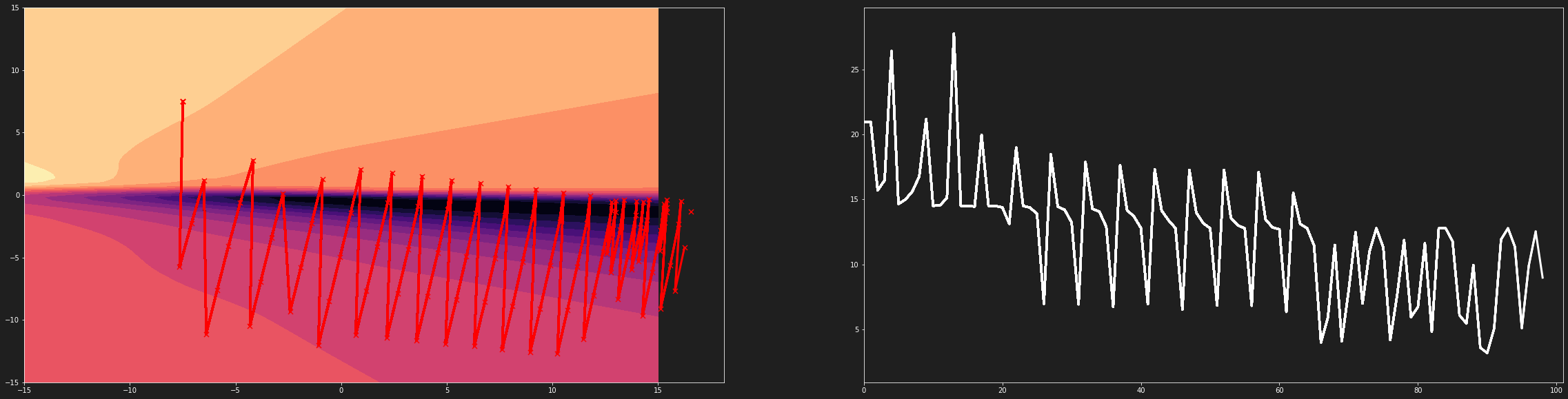
def animate(params):
  W0 = params[0]
  W1 = params[1]
  b = params[2]
  i = params[3]
  loss = params[4]
  

  # ax[0].clear() # frontiere de décision
  # ax[1].clear() # sigmoide
  # ax[2].clear() # fonction Cout
  
  ax[0].contourf(W11, W22, L, 20, cmap='magma', zorder=-1)
  ax[0].scatter(Params1[int(i)], Params2[int(i)], c='r', marker='x', s=50, zorder=1)
  ax[0].plot(Params1[0:int(i)], Params2[0:int(i)], lw=3, c='r', zorder=1)

  ax[1].plot(Loss[0:int(i)], lw=3, c='white')
  ax[1].set_xlim(0, len(Params1))
  ax[1].set_ylim(min(Loss) - 2, max(Loss) + 2)

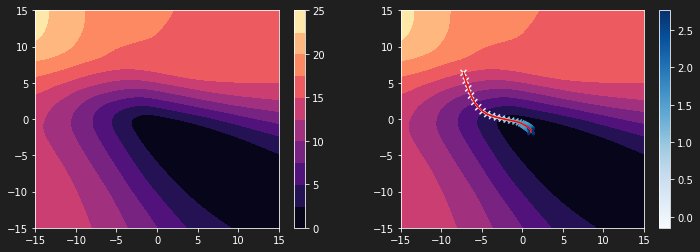
plt.figure(figsize=(12, 4))
plt.subplot(1, 2, 1)
plt.contourf(W11, W22, L, 10, cmap='magma')
plt.colorbar()

plt.subplot(1, 2, 2)
plt.contourf(W11, W22, L, 10, cmap='magma')
plt.scatter(history[:, 0], history[:, 1], c=history[:, 2], cmap='Blues', marker='x')
plt.plot(history[:, 0], history[:, 1])
plt.plot(history[:, 0], history[:, 1], c='r')
plt.colorbar()

<matplotlib.colorbar.Colorbar at 0x7f07d39a2790>

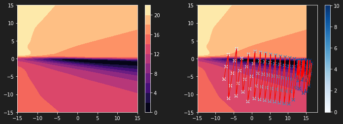
The graph above shows that the steps of our algorithm are not adjusted to our loss function. The latter is much too compressed. It is thus difficult to reach the global minimum.

Creation of an animation

Let’s make a video representing the evolution of the previous curve while the descent occurs on our loss function.

fig, ax = plt.subplots(nrows=1, ncols=2, figsize=(40, 10))
ani = FuncAnimation(fig, animate, frames=history, interval=10, repeat=False)

import matplotlib.animation as animation
Writer = animation.writers['ffmpeg']
writer = Writer(fps=10, metadata=dict(artist='Me'), bitrate=3200)
ani.save('animation3.mp4', writer=writer) ## To store the animation locally

Gradient descent on a compressed loss function

3D Visualization of Loss function

import plotly.graph_objects as go

fig = (go.Figure(data=[go.Surface(z=L, x=W11, y=W22, opacity = 1)]))

fig.update_layout(template= "plotly_dark", margin=dict(l=0, r=0, b=0, t=0))
fig.layout.scene.camera.projection.type = "orthographic"
fig.show()

ii. Case of normalized inputs data

Create a dataset

In the latter, also generated with the make_blobs function, the data have the same order of magnitude.

from sklearn.datasets import make_blobs

X, y = make_blobs(n_samples=100, n_features=2, centers=2, random_state=0)
X[:, 1] = X[:, 1] * 1
# X[:, 1] = X[:, 1] * 10

y = y.reshape(y.shape[0], 1)

plt.scatter(X[:,0], X[:, 1], c=y, cmap='ocean')
plt.show()

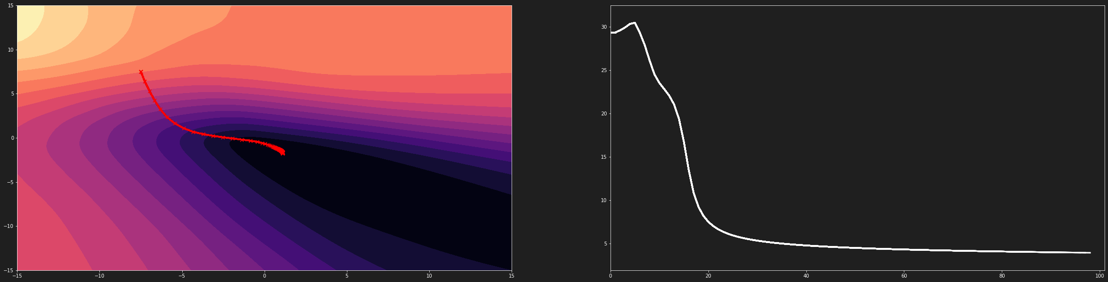
Visualize the learning curve

Using the same artificial neuron, we obtain the following diagram which is “uniform” (cqfd)

Visualize Gradient Descent

On the following diagram, the gradient descent algorithm has a suitable evolution

Gradient descent on an uncompressed loss function

3D Visualization of Loss function

Conclusion

If one of the parameters has much more influence than the second, then the cost function will be “compressed” making convergence difficult and multiple overflow errors. When the variables are on the same scale, the cost function evolves in a similar way on all its parameters. This allows a good convergence of the gradient descent algorithm

Links

Getting The Code On Google Colab

The entire code containing all the code mentioned in this post can be found here.

Getting The Code On Github

The entire folder containing all the code mentioned in this post can be found via this link.

Just bear in mind that you will need to install all the dependencies. If you find any issues with the code, feel free to either comment down below or raise an issue on Github.

Add me on LinkedIn

Don’t hesitate to follow me on linkedIn or o other social network to encourage me to do more posts on IT.